การทำงานในช่วงเดือนกันยายน

(อัพเดตเมื่อวันที่ 5 ตุลาคม)

ทำการศึกษาโค้ดเกี่ยวกับ I2S ที่เคยมีคนทำมาแล้ว

ได้ใช้โค้ดจาก dronebotworkshop เพื่อทำการทดลองการใช้งาน โดยตัวของโค้ดมีหลักการทำงานของโค้ดคร่าวๆ ดังนี้

• ทำการอ่านค่าจากฟังก์ชัน i2s_read 1 ครั้ง
• หาค่าเฉลี่ยของ input ที่อ่านได้ใน buffer ตั้งแต่ buffer[0] จนถึง buffer [7] ( 8 ตัว )
• แสดงผลค่า mean ผ่าน serial plot บน Arduino IDE

และมีการทำ I2S setting parameters ดังนี้

• buffer length = 64 (buffer ชนิด int16_t สามารถเก็บข้อมูลขาด 2 bytes ได้ตรงกับ bit resolution พอดี)
• sample rate = 8000 Hz
• bits_per_sample = 16 bits

โดยมีตัวอย่างโค้ดการทำงาน ดังนี้

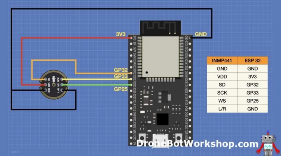
// Connections to INMP441 I2S microphone
#define I2S_WS 25
#define I2S_SD 33
#define I2S_SCK 32
// Use I2S Processor 0
#define I2S_PORT I2S_NUM_0
// Define input buffer length
#define bufferLen 64
int16_t sBuffer[bufferLen];
void i2s_install() {
// Set up I2S Processor configuration
const i2s_config_t i2s_config = {
.mode = i2s_mode_t(I2S_MODE_MASTER | I2S_MODE_RX),
.sample_rate = 8000,
.bits_per_sample = i2s_bits_per_sample_t(16),
.channel_format = I2S_CHANNEL_FMT_ONLY_LEFT,
.communication_format = i2s_comm_format_t(I2S_COMM_FORMAT_STAND_I2S),
.intr_alloc_flags = 0,
.dma_buf_count = 8,
.dma_buf_len = bufferLen,
.use_apll = false
};

i2s_driver_install(I2S_PORT, &i2s_config, 0, NULL);
}

void i2s_setpin() {
// Set I2S pin configuration
const i2s_pin_config_t pin_config = {
.bck_io_num = I2S_SCK,
.ws_io_num = I2S_WS,
.data_out_num = -1,
.data_in_num = I2S_SD
};
i2s_set_pin(I2S_PORT, &pin_config);
}
void setup() {
// Set up Serial Monitor
Serial.begin(115200);
Serial.println(" ");
delay(1000);
// Set up I2S
i2s_install();
i2s_setpin();
i2s_start(I2S_PORT);
delay(500);
}
void loop() {
// False print statements to "lock range" on serial plotter display
// Change rangelimit value to adjust "sensitivity"
int rangelimit = 3000;
Serial.print(rangelimit * -1);
Serial.print(" ");
Serial.print(rangelimit);
Serial.print(" ");

// Get I2S data and place in data buffer
size_t bytesIn = 0;
esp_err_t result = i2s_read(I2S_PORT, &sBuffer, bufferLen, &bytesIn, portMAX_DELAY);

if (result == ESP_OK)
{
// Read I2S data buffer
int16_t samples_read = bytesIn / 8;
if (samples_read > 0) {
  float mean = 0;
  for (int16_t i = 0; i < samples_read; ++i) {
    mean += (sBuffer[i]);
  }

  // Average the data reading
  mean /= samples_read;

  // Print to serial plotter
  Serial.println(mean);
}
}
}

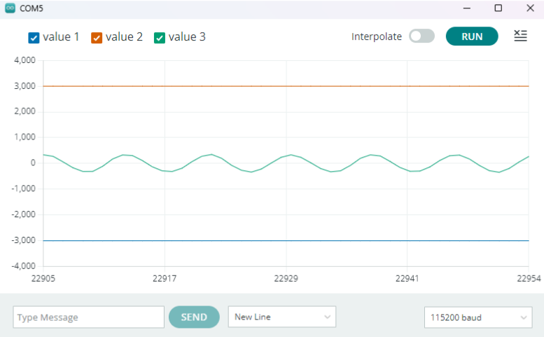
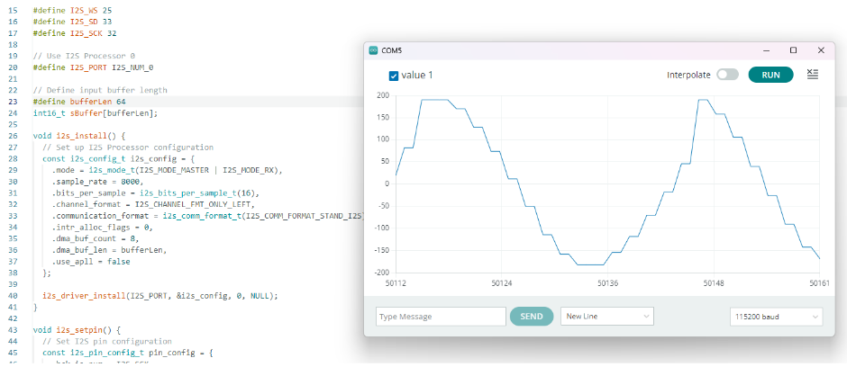
ผลลัพธ์การทดลอง

จากนั้นจะได้ผลลัพธ์จากการนำ input 220Hz ผ่าน speaker ของโทรศัพท์มือถือเพื่อทดสอบสัญญาณ โดยใช้คลื่นความถี่เสียงจากคลิป คลื่นความถี่เสียง A 220Hz โดยจะแสดงออกมาเป็นรูปกราฟ ดังนี้

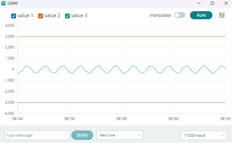
ผลลัพธ์จากการนำ input 440Hz ผ่าน speaker มือถือเพื่อทดสอบสัญญาณ โดยใช้คลื่นความถี่เสียงจากคลิป [คลื่นความถี่เสียง A 440Hz] (https://youtu.be/OUvlamJN3nM?si=fY32C0fwpD0X4YNQ)
โดยจะแสดงออกมาเป็นรูปกราฟ ดังนี้

ข้อสังเกตจาก output ของโค้ดของ dronebotworkshop

• output ที่ได้ มาจากค่า mean ของ ค่าใน buffer 8 ตัว ( มาจาก bytesIn = 64 , ทำการ for loop ใน byteIn/8 = 8 ตัว) ทำให้ค่าที่ได้ เป็นค่าจากการรวมกันของข้อมูล ไม่ใช่ค่า ณ เวลานั้นๆ
• การ plot บน serial plot นั้นยังไม่สามารถบอกความสัมพันธ์ระหว่างค่าที่ได้กับเวลาจริงๆ ( การ plot บน serial plot ทำการ plot โดยมี แกน X คือ Baud rate ซึ่งเราไม่สามารถนำไปบอกความสัมพันธ์ได้ ว่ากราฟที่ได้ ใช่กราฟความถี่ที่ถูกต้องตาม input หรือไม่)

ทำการแก้ไขโค้ด เพื่อแสดงผลค่า buffer ทุกตัวมาดู จะได้ดังนี้

for(int i=0;i<bytesIn;i++){
  Serial.println(sBuffer[i]);
  //Serial.print(",");
}
Serial.println("");

ทำให้พบว่า ค่าใน buffer 32 ตัวแรกนั้นสามารถอ่านค่าได้ แต่ค่า 32 ตัวหลังนั้นเป็น 0 ทั้งหมด สาเหตุมาจาก การตั้ง Format ของข้อมูลเป็น I2S_CHANNEL_FMT_ONLY_LEFT , และจากการที่ทำการต่อ pin L/R เข้ากับขา ground ของวงจร ดังรูป

ทดลองนำโค้ด I2S มาปรับใช้กับงานที่ทำ ดังนี้

for(int i=0;i<bytesIn/2;i++){
  Serial.println(sBuffer[i]);
  //Serial.print(",");
}
Serial.println("");

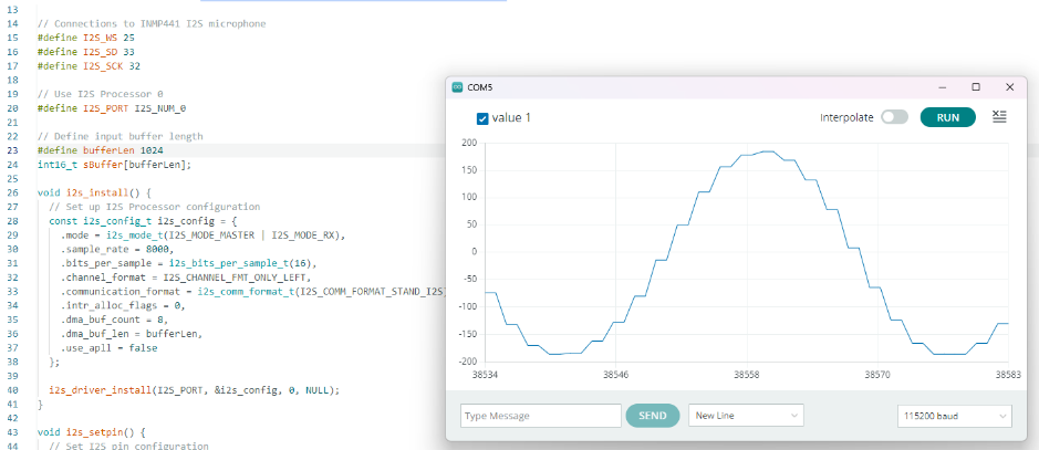
ทำการปริ้นค่าใน buffer ไปจนถึง bytesIn/2 ( ตัด 32 ตัวหลังที่เป็น 0 ออก ) และทำการเปรียบเทียบรูปกราฟคร่าวๆ ระหว่างการใช้ buffer length 64 กับ 1024 โดยมี Input เป็นความถี่ที่ 220Hz ดังรูป

ทดลอง เพิ่มค่า buffer length เป็น 1024 จะได้ผลลัพธ์ดังนี้

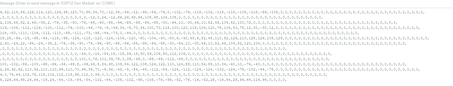
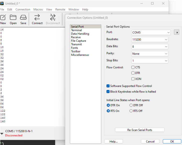
ทดลองการอ่าน Serial monitor เพื่อ save ข้อมูลไปยัง text file

โดยมีการใช้โปรแกรม Coolterm เพื่อทดสอบ ศึกษาพื้นฐานการใช้งานจาก How to Save Arduino Serial Data in TXT, CSV and Excel File

ตัวอย่างการใช้งาน Coolterm

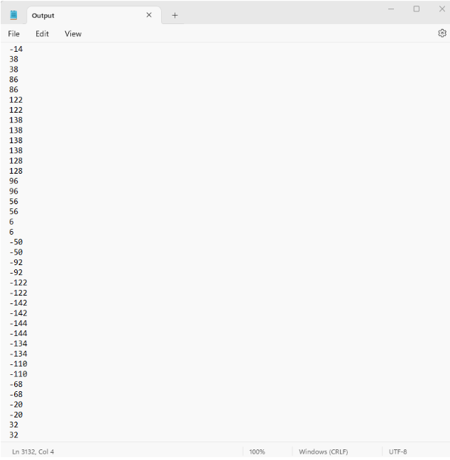
ตัวอย่างข้อมูลที่เก็บได้

ตัวอย่างโค้ด python ที่ใช้ในการ plot ข้อมูลที่ได้

audio_data = []

with open("Output.txt", "r") as file:
for line in file:
  line = line.strip()
  if line:
      try:
          audio_data.append(int(line))
      except ValueError:
          print(f"Skipping invalid line: {line}")

# Define the time range you want to display (e.g., 10 ms)
start_time = 1  # Start time in seconds
end_time = 1.02  # End time in seconds (10 ms)

# Find the corresponding indices in the audio data
sampling_rate = 8000
start_index = int(start_time * sampling_rate)
end_index = int(end_time * sampling_rate)
audio_data_subset = audio_data[start_index:end_index]

# Create the time axis for the subset
time_axis = [i / sampling_rate for i in range(start_index, end_index)]

# Define the specific times where you want to point
point_times = [1.0040, 1.0085,1.0131]

# Plot the audio data subset
plt.figure(figsize=(10, 4))
plt.plot(time_axis, audio_data_subset, linewidth=0.5)
plt.xlabel("Time (s)")
plt.ylabel("Amplitude")
plt.title(f"Audio Data ({start_time} to {end_time} seconds)")
plt.grid(True)

# Add points and annotations
for point_time in point_times:
# Find the index corresponding to the point time
point_index = int(point_time * sampling_rate)

# Get the amplitude at that index
point_amplitude = audio_data_subset[point_index - start_index]

# Annotate the point on the plot
plt.annotate(f"({point_time:.4f}, {point_amplitude})", xy=(point_time, point_amplitude),
           xytext=(point_time + 0.001, point_amplitude + 0),  # Adjust text position
           arrowprops=dict(arrowstyle="->", lw=1.5, color='red'),
           fontsize=10, color='red')

plt.show()

จะได้ผลกราฟจากการ plot ดังนี้

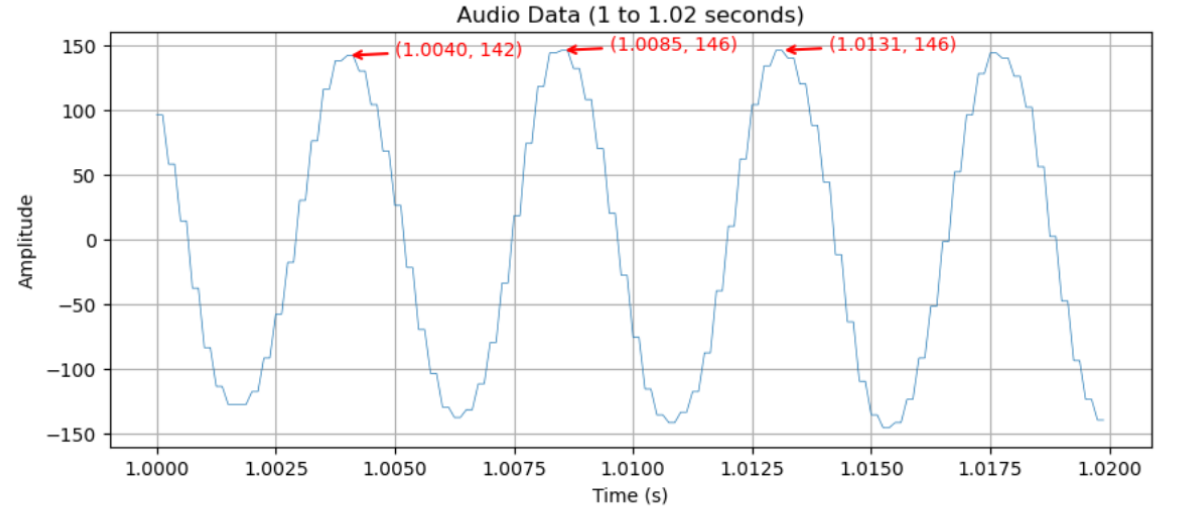
จะเห็นได้ว่า ช่วง peak-peak นั้น มีเวลาต่างกัน 1.0085 - 1.0040 = 0.0045 second ซึ่งเป็นคาบของคลื่นนี้ และทำการหาความถี่จะได้ 1/0.0045 = 222.22 Hz ซึ่งตรงกับ Input ที่ได้ทำการป้อนเข้าไปนั่นเอง